The upshot: MLPerf has announced inference benchmarks for neural networks, along with initial results.

Congratulations! You now have the unenviable task of deciding which neural-network (NN) inference engine to use in your application. You want, of course, the fastest one. And it needs to run at the edge on a battery-powered device. All you have to do is compare all of the options out there to see which works best!

But here’s the thing: there’s an enormous amount of variability in how neural networks perform across different platforms. This is particularly true when you consider that some platforms are more appropriate for cloud inference, while others target line-powered edge applications, and still others focus on battery-powered applications.

Even on a specific platform, designers may optimize a model differently in an attempt to get the best power-performance point without sacrificing too much accuracy. When benchmarking microprocessor, such fiddly adjustments raise a suspicion of manipulation, of rigging the results. But, with NN development, such optimizations reflect the real world, not some made-for-benchmark exception. As usual, it’s a game of tradeoffs.

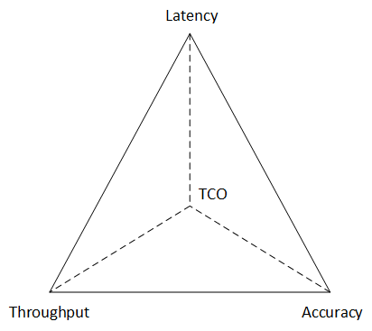
I’ve noticed more than one of the “pick-two” feature triangles, each involving latency and/or throughput and/or accuracy and/or total cost of ownership (TCO). With any of these triangles, you can improve two of the parameters at the expense of the third. I then realized that those triangles were all sides of a tetrahedron that gives a “pick-three” relationship. In other words, if you’re willing to sacrifice one variable, you can improve three others. The pick-two triangles tacitly assume that the fourth variable is static.

In a study of the relationship between accuracy and computing power across a variety of architectures done at the Universita degli Studi di Milano-Bicocca, a team graphed accuracy as a function of putative computing strength, as measured in Giga-floating-point operations, or GFLOPs. Yes, the least accurate solutions had the lowest GFLOPS, and the highest accuracy was achieved using the most GFLOPS, but, in between, there’s a huge amount of variability that hurts the accuracy/performance correlation.

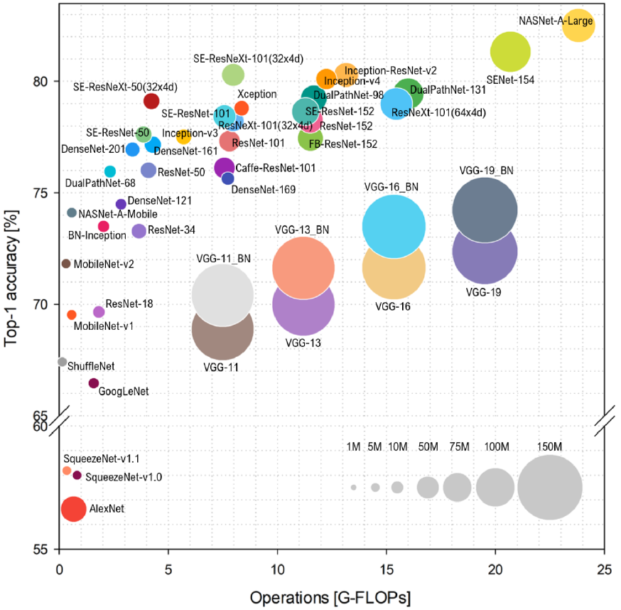
(Click to enlarge. Image credit: Bianco, S., Cadene, R., Celona, L., and Napoletano, P., Benchmark Analysis of Representative Deep Neural Network Architectures. IEEE Access, 6:64270–64277, 2018, via MLPerf)

So, given all of these possible variations, is it even possible to find some neutral way to compare inference engines? Might a credible set of benchmarks be possible where vendors and customers can come together to share results?

MLPerf thinks so – not surprising, since they’ve already released a set of NN-training benchmarks. In their paper introducing the new benchmarks, they cite all of the above reasons and relationships as serious challenges to a set of universal – or at least widely applicable – benchmarks.

Inference benchmarks are not simply a tweak of training benchmarks – the metrics used are completely different. With training, you’re concerned about how long it takes to train a model to a given level of accuracy. By definition, that process involves many passes through the network with back-annotations on the weights until the model converges. That process has no applicability in the inference world, where each inference involves a single pass forward through the network (with possible loops along the way if it’s a recurrent network).

MLPerf has addressed the issue of optimizations by defining these as semantic-level benchmarks: “Here’s the task you must perform, and here’s the model you must use. Implement it the best way you can on your architecture and submit the results.” That makes optimization fair game – even though two different teams optimizing for the same architecture might use different approaches and get different results.

The middle ground that MLPerf has had to find is captured in the following five principles*:

“Pick representative workloads that everyone can access.
Evaluate systems in realistic scenarios.
Set target qualities and tail-latency bounds in accordance with real use cases.
Allow the benchmarks to flexibly showcase both hardware and software capabilities.
Permit the benchmarks to change rapidly in response to the evolving ML ecosystem.”

The fourth one in particular allows a submitter (who is usually the vendor of an architecture) to submit multiple variations, if relevant, with certain limitations in how the reporting is done (we’ll return to that).

Benchmarking Setup

The benchmark architecture is intended to provide modularity, flexibility, and re-use as shown below. The model and the system-under-test (SUT) are separate entities so that they can be readily substituted. How the benchmarking proceeds is determined by the Load Generator, commonly abbreviated LoadGen. Any changes to setup or scenario are reflected there, independently of the model and SUT. The “Accuracy Script” accepts output logs from LoadGen to confirm results.

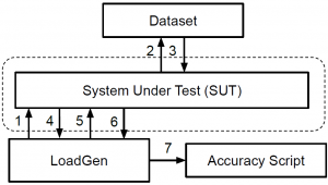
(Image courtesy MLPerf)

There are four main scenario settings that LoadGen handles:

Single-stream; critical metric is latency (90th percentile). This represents a common real-time scenario, where latency – the time it takes to do a single inference – is critical. It’s also sometimes referred to as “batch=1”: each inference must be completed before the next inference starts. A typical example of this would be a security video feed, where each frame must be processed entirely before the next frame arrives. The flow here is strictly sequential; a new query isn’t submitted by LoadGen until the previous one is complete.
Multi-stream; critical metric is the number of streams that can be managed for a given latency. This scenario is typical of an automotive application where multiple camera and other streams must be processed and correlated together. Here the queries are submitted at a given interval; if the prior query isn’t complete when a new one is scheduled, then the new one is dropped. Only 1% of samples can be dropped.
Server; critical metric is the number of queries per second (QPS) at a given quality of service (QoS) – i.e., latency – level. This scenario reflects online queries whose arrival times will be random. Those arrivals are scheduled using a Poisson distribution whose parameters can be set in LoadGen. No more than 1% of the queries (3% for a translation application) can exceed the latency limit.
Offline; critical metric is throughput. This represents a high-batch scenario where, for example, a company is running through a series of images that are all immediately available in storage. Inference here can be optimized, for instance, by running all of the images through one NN layer before loading the weights for the next layer. That would mean storing the activations for each layer so that they can be retrieved when the next layer operates. This minimizes the moving of weights – but in a way that works only for offline processing, not for stream processing. Batches must have at least 24,576 samples.

The latency restrictions are more specifically referred to as tail-latency. The idea here is that there’s often a certain degree of stochastic behavior, so there’s always a random chance of an outlier. The latency restrictions set the percentage of latency results that can fall within this tail.

The benchmarks themselves specify 5 different models and three different tasks, as shown in the following table. Each task has a dedicated model, with two of the tasks having both heavy- and light-duty versions. The specific data sets to be used are also fixed, as is the quality target.

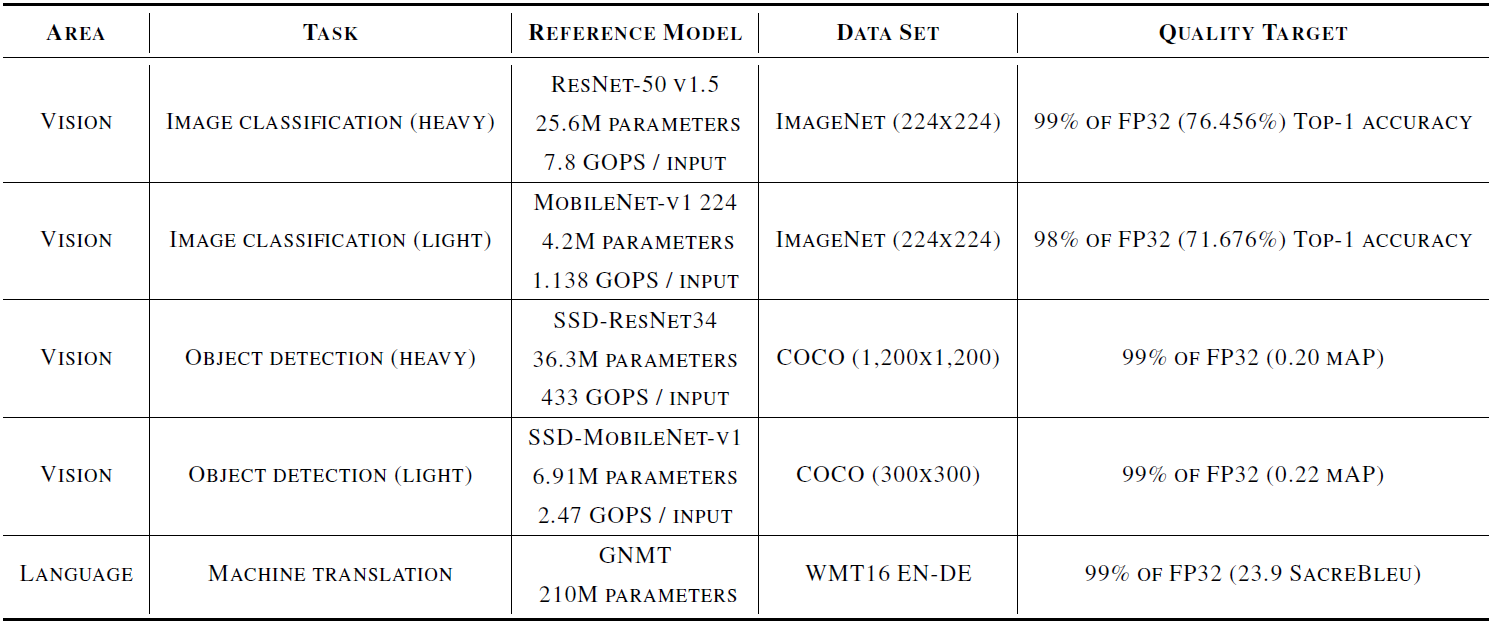
(Click to enlarge; image courtesy MLPerf)

Note that the quality targets refer only to the accuracy achieved through the inference process. The reference models are 32-bit floating-point models; this sets the accuracy targets for optimizations done on the models to ensure that they aren’t “optimized” to such an extent that accuracy suffers simply for the sake of speed and a good benchmark result.

There is also a reference to mAP, or mean average precision, on some of them. This refers to an average of the achieved precisions across the data set, as described more precisely here. Others refer to “top-1 accuracy.” This gets to what you might think of as the “top-n” possible results, since the inference result isn’t always certain. If it were “top-5,” that would mean that the right answer was in the top 5 most likely results. For top-1, it means that the most likely result must be the correct result; you can find more details here. Finally, the translation task makes reference to SacreBleu – a way of evaluating translation results.

Reporting Considerations and Results

MLPerf has provided both for a means of comparing different architectures as well as for a means of showing what more creative implementations might achieve. This is done through two divisions: open and closed.

The closed division reflects more of what we would expect of a benchmark when comparing inference engines. The specified models (or equivalent) and data sets must be used, constrained by the quality targets above. Pre- and post-processing are specified. One can quantize and calibrate the models using their calibration data sets. No retraining is allowed.

The open division may show more of what a specific engine can do, but results can’t be readily compared between submissions. Submitters must perform the specified tasks, but they can use their own pre- and post-processing, change the data sets, vary the models, and do retraining. But they must document all of the ways in which they deviate from the closed-division requirements.

Architectures are to be reported in one of three categories:

Available: hardware and software must be commercially available according to specific requirements.
Preview: hardware and software must be staged for availability within 180 days or the next submittal deadline, whichever is farthest out.
Research: this is intended more for leading-edge architectures that might not be intended for commercial release.

The results of the latest round of submissions (for the 0.5 version) are summarized in the graphic below, with much more detail laid out in MLPerf’s research paper. This reflects the result of over 600 submissions for this particular round. Note that the results have all been normalized to the slowest implementation. Nvidia has separately claimed that they won all five categories and that they were the only company to submit results for all five tasks.

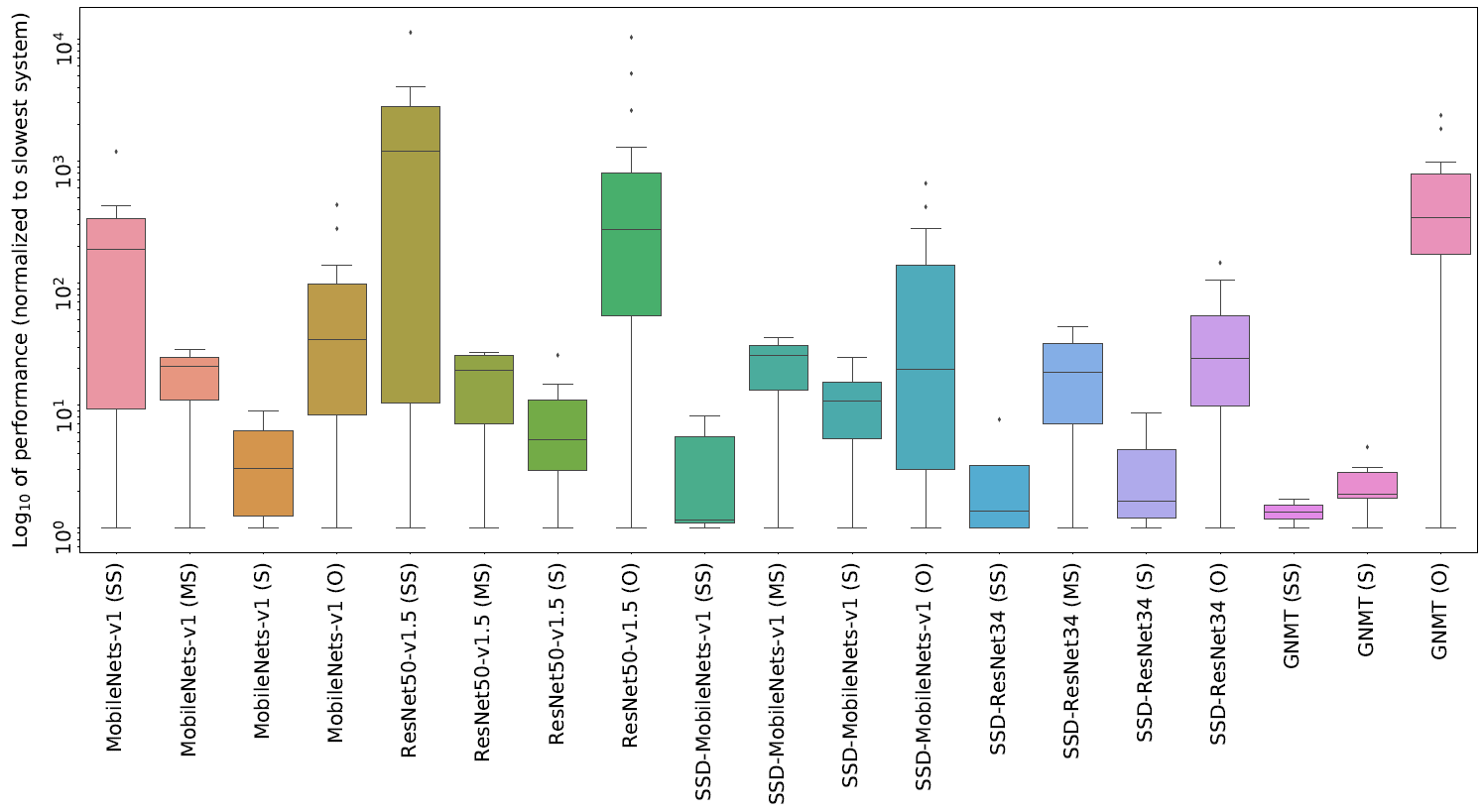
(Click to enlarge; image courtesy MLPerf)

It’s worth noting that this isn’t the first attempt at NN benchmarks. In their paper, MLPerf addresses how their new benchmarks compare (qualitatively) with several prior efforts: AI Benchmark, EEMBC MLMark, Fathom, AIXPRT, AI Matrix, DeepBench, Training Benchmark for DNNs (“TBD”), and DawnBench.

So, do we now have a set of benchmarks on which everyone can agree? Well, we’ve undoubtedly made progress. I happened to have a conversation with Flex Logix CEO Geoff Tate, and Flex Logix is very supportive of the work that MLPerf is doing. But the request that they get most commonly from their potential customers is for performance on YOLO v3, with 1 megapixel samples being the smallest size requested. Raising the size of models has non-linear implications: he said that doubling ResNet50 changes activation size from 1 Mb to 50 Mb, so results from larger models aren’t easily extrapolated from smaller ones. If MLPerf included a 2-megapixel YOLO v3 model, “they’d be all over it.”

Another caution about NN benchmarks in general comes from Blaize, about whom we recently wrote. While there’s intense interest in the performance of NN inference engines, they note in a whitepaper** that the inference engine may not be the bottleneck. In a complete vision pipeline, for example, the pre- and post-processing steps may, in fact, run slower than the inference. In such a situation, one might end up paying more for a faster inference engine, only to find that the extra cost hasn’t bought any higher system performance.

One final thought relates to the impact of NN development software. We’ve seen before the need to quantize, prune, fuse, and retrain networks. Some tools do these tasks automatically; some support manual execution of these optimizations, with automation on their roadmaps. Automation not only saves design time; it also makes NN development accessible to more engineers who don’t have to study the intricacies of all these different ways of tweaking the design.

So it would be interesting if the benchmark suite at some point offered “push-button” and “hand-optimized” categories. The thought here is that vendors of inference engines can well afford to invest in lots of effort to make their engines look good, and they’ll probably use experts to do that. That’s fine, but they may spend more effort than your average design budget would allow. So, seeing what’s possible using automated tools – even if you can do even better using further hand tweaks – would seem to have some value.

*Source: MLPerf Inference Benchmark, V.J. Reddi et al.

** Requires email submittal to receive whitepaper.

More info:

MLPerf Inference benchmarks

Sourcing credit:

Itay Hubara, Research Scientist, Habana (under acquisition by Intel), Contributing Member of MLPerf

Paresh Kharya, Director of Product Management, Nvidia