[Editor’s note: this piece has been updated at the end.]

Cadence recently announced neural-network processor IP. It would be pretty simple to jump into the architecture and start from there, but there’s this thing that I don’t think is just me that perhaps we should deal with first.

I see neural networks tossed about all over the place. In none of those places is there ever a description of what neural networks are – in their various embodiments. So either it’s experts talking to experts, or everyone is doing a good job of pretending to know this stuff.

But the thing is, if something like that might be useful but you have to embarrass yourself by raising your hand and saying, “Excuse me sir/ma’am, but could you please back up and explain just what the heck you’re talking about?” then you might instead opt to forego investigating the technology. It’s easy to say, “Oh, they don’t apply to what I’m doing,” and leave it at that.

Well, this is me raising my hand – or was me, until I did some digging. So before we discuss the specifics of Cadence’s processor, there are a number of notions that we should clear up first, foremost being neural nets – in particular, convolutional neural nets (CNNs) and recurrent neural nets (RNNs). We’ll make this brief – but hopefully not too brief. For those of you who saw last week’s piece on Solido’s machine learning, we did some basic background on higher-level machine-learning concepts, but this will take the platforms on which such algorithms run into more detail.

Neural Net Review

Let’s start with the notion of the perceptron. There appears to be some pedantic disagreement as to whether this is a node in a network or just a really simple network (with one node), but it’s a basic unit however you think of it. It has a bunch of inputs and a single output. The inputs are each multiplied by some weight, after which an activation function is applied. In this case, it would be a linear function.

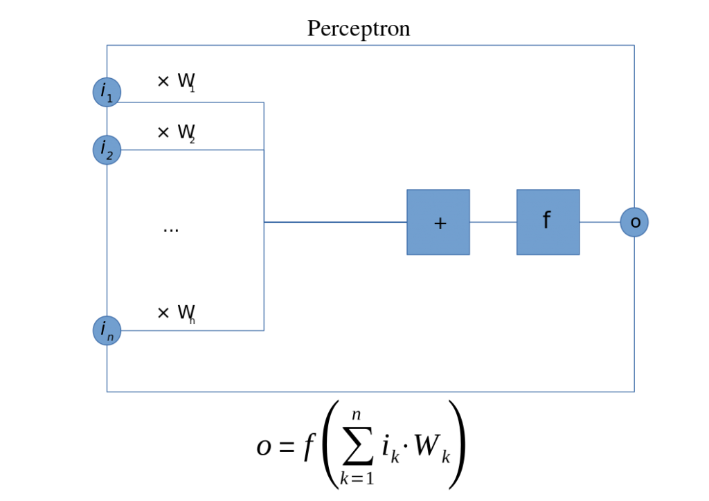
(By Mat the w at English Wikipedia, CC BY-SA 3.0)

This can be used for basic classification. In a learning context, the weights are adjusted as the system learns; this amounts to a model being tweaked until it presents the correct answer for any case where the correct answer is known. From this, you then have faith that it will also generate the correct answer for any case where you don’t know the correct answer.

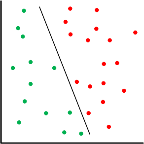
Based on the linearity thing, this amounts to a case where the “divider” in a one-or-the-other classification is a line.

A basic network has input and output nodes – two layers. A multi-layer perceptron has additional layers; the layers between input and output are referred to as hidden layers. This makes it a deep neural network. In this case, some of the activation functions may be nonlinear. A common type of non-linear function is a sigmoid, so-called because they look sort of like an S. The idea here is that, for classification, it acts as something of a threshold function, with a narrow ambiguous region and the rest clear in-or-out, approximating a step function.

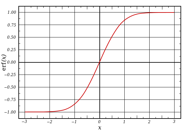
(Example sigmoid: the error function. Source: Wikipedia)

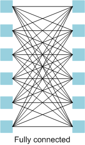
A multi-layer perceptron is a fully-connected network. This means that each layer is fully connected, which means that it has each node fed by all inputs from the prior layer.

A feed-forward network is pretty self-explanatory: all signals proceed through the network from (using Western convention) left to right. A recurrent neural network (RNN – not to be confused with a recursive neural network), however, has feedback, so it’s not feed-forward. From a dataflow standpoint, feed-forward networks are described by directed acyclic graphs (DAGs); RNNs are cyclic.

Natural-language, speech, and handwriting recognition and other time-varying phenomena tend to benefit from RNNs. I haven’t dug in far enough to know exactly why that is; off the top of my head, my guess would be that the feedback provides for storage of state. For vision processing, however, we turn to biology to point us in the right direction.

I C U

It turns out that you have multiple neurons in your eyes, and each one handles a particular tile of your visual field. The tiles overlap somewhat; together you get the entire field. The way each tile is processed by the neuron turns out to be very similar to convolution.

Yeah, I know. Convolution. It’s that odd mathematical function that, at least for some of us, was presented as some strange integral with no rationale. We simply memorized it like dutiful drones (and some of us regurgitated on the final, correctly or not, and forgot it) and moved on. It becomes multiplication in the s-domain. Yay.

Simplistically, I think of it as a complex cross product of a couple of fields. You slide one function across another function, multiplying and summing to get yet a third function. Wikipedia has some helpful graphics and animation.

This is where the notion of the convolutional neural network, or CNN comes from. CNNs have different types of layers; they’re not all convolutions and they’re mostly not fully connected. The convolutional layers do exactly what it sounds like, with each input node in a layer getting a tile from the original image. All of the nodes in the layer have the same weights for their inputs.

Then there’s often a pooling layer, where the convolutional results are down-sampled to reduce the field size. One way that’s done is by tiling up the convolution results for a particular original tile (yes, tiling up the tile) and picking the maximum value within the tile; this value represents the entire original tile. If the new tile (within the original tile) is 2×2, you’ve now down-sampled by a factor of 4.

This may be followed by more convolutional and pooling layers. Towards the end (where the volume of data has been greatly reduced), there is often a fully connected layer driving the final result. The following drawing shows a generalized view, where the subsampling is performed by the pooling layers.

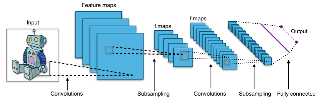
(By Aphex34 – Own work, CC BY-SA 4.0)

So How Do You Do One?

OK, so that’s a super brief primer, at least according to my understanding. If you’re actually trying to use something like this, how do you do it? There are a couple of layers to that answer. (Of course.) At the highest level, you describe the learning behavior that you want to implement. There are some tools available to abstract this design, most notably Caffe, a deep learning framework from UC Berkeley, and TensorFlow, a dataflow tool started by Google and open-sourced last year. This is mostly where you want to play, because you can focus at a higher level on the nature of your network and the problem you’re trying to solve.

What you describe up top, of course, has to be implemented somehow on some processing platform, and there are lots of options for this. You can use CPUs, GPUs, DSPs, and any combination thereof. But it’s all pretty computationally intensive – especially the convolutional part, so folks have opted to accelerate that with dedicated chips. In that configuration, you have a CPU acting as a host processor; it hands off convolutional duties to the accelerator.

The big challenge is that, as the processing passes back and forth between the processor and the accelerator, the data has to move along with it. Much effort is expended in the movement of data.

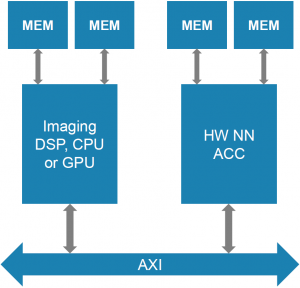
(Image courtesy Cadence)

Movidius is an example of a company that has put together a deep-learning chip; they were a high flyer and were bought by Intel. They’ve got a dedicated “SHAVE” vector engine along with a couple of CPUs and dedicated hardware for sparse data structures; it’s a mixed software/dedicated hardware solution. They claim teraFLOP performance with 1 W of power dissipation.

Which brings us to what Cadence has announced, via their Tensilica arm. Unlike Movidius, they’re not selling an actual chip; they’re selling IP: the Tensilica Vision C5 DSP. They’ve taken the notion of convolution acceleration one step further into a processor that can handle all of the layers of a CNN, not just the convolutional layers. As a result, the intent is that you can do everything with a single DSP, rather than using two processing blocks. As a result, data doesn’t have to move between a host and an accelerator.

They’ve broken down the challenges with alternative implementations as follows:

• CPUs, while familiar and easy to use, with future-proofing via updates (as long as you stay in the memory footprint), use too much power and achieve less than 200 GFLOPs performance.
• GPUs do a little better on the power front, but not great; they achieve around 200 GFLOPs.
• They see accelerators as less flexible (due to various bits of fixed hardware, which gives them pause in a rapidly evolving field like this) and harder to use because you need to separate the software bits from the hardware bits. They do well on power and can achieve greater than 1 TMAC, but the dedicated hardware limits future-proofing options. Data movement also gets in the way. From a performance standpoint, here we’re comparing TFLOPs to TMACs, which Cadence says you can’t do because it depends on the MAC precision. But performance is performance, and if you want to compare the two solutions, what to do? My personal instinct, precision aside, is that a FLOP – one floating-point operation – is less performance than one MAC – involving multiplies and addition.
• A simpler vision-oriented DSP (like the Tensilica Vision P6) gets the ease of design, power, and future-proofing down, but manages only 200-250 GMACs.

The C5 block diagram looks like the following. (Yeah, there’s an extra Load block in the memory path; I confirmed that it’s correct, but I don’t have an explanation on what that does vs. the Load/Store block [Editor’s note: see update below]).

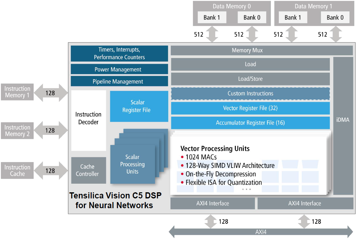
(Image courtesy Cadence)

They use two memories – one for read; one for write. When one layer is complete, they reverse the direction, ping-ponging to keep from having to move the data.

The processing is pretty extensive; it’s a 4-way VLIW 128-way SIMD processor. Let’s unpack that. SIMD, of course, means single-instruction/multiple-data. In this case, you have 128 values that will all be operated on by the same instruction, in parallel.

But where SIMD gives you data parallelism, VLIW gives you instruction-level parallelism. It stands for very-long-instruction-word, and it’s so long because it contains some number – in this case, 4 – of instruction/data pairs. Each of the instructions can be (and probably is) different. So here you can do four different things all at once. What’s notable in this case is that the data isn’t necessarily just a value or scalar; it can be a 128-bit vector. So you get four SIMD instructions in parallel, meaning that you’re doing 1024 operations at the same time. (Hence the 1024 MACs, presumably.)

They can also scale in a multi-processor configuration with shared memory, as shown below. Yeah, they look like separate memories, but they have a way of sharing them. Perhaps it’s more like a single memory distributed amongst the cores.

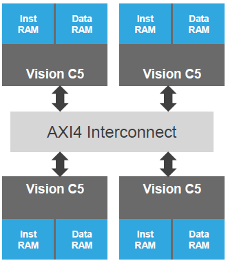
(Image courtesy Cadence)

All in all, they use the following image to illustrate their view of the advantages of the C5 vs. accelerators. Note that this processor can be used as a complement to an imaging DSP, but, if so, the imaging DSP doesn’t share any of the neural network burden; that’s handled entirely within the C5 DSP.

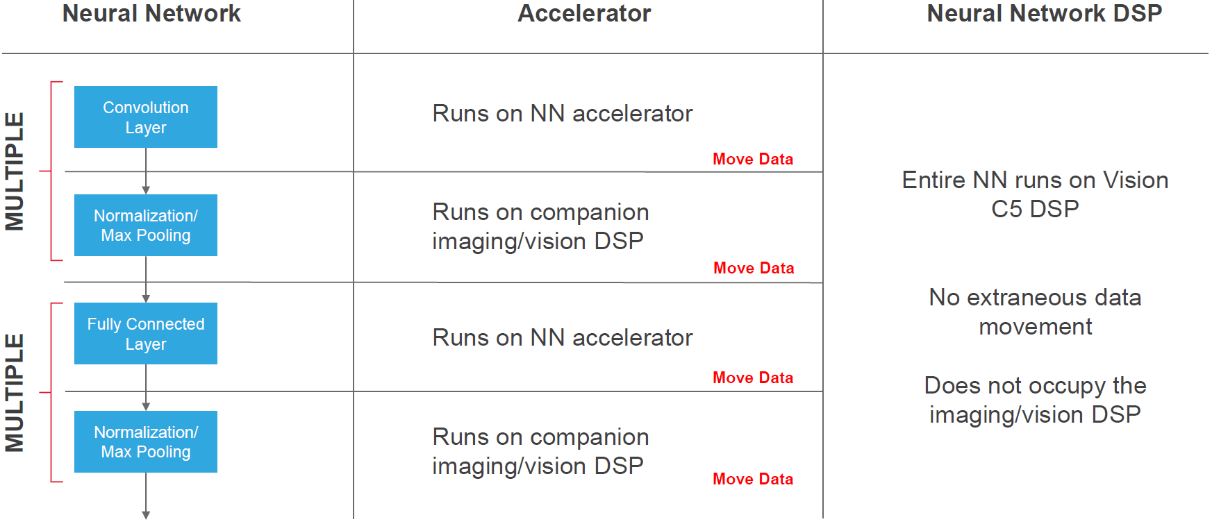
(Image courtesy Cadence)

The last thing to look at is, what does the design flow look like? As mentioned before, you’d really like to keep your work within the high-level frameworks (e.g., Caffe/TensorFlow). That would appear to be supported by Cadence’s development kit.

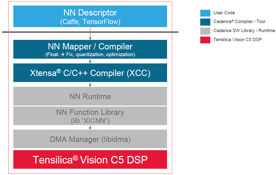
(Image courtesy Cadence)

So that’s a quick run-down of the Cadence neural-net IP. As an additional angle on the topic, a dedicated CNN-RNN processor was presented at ISSCC earlier this year by KAIST in Korea. They note that convolutional layers, recurrent layers, and fully connected layers may coexist in a network, but they have very different processing requirements. Convolution requires lots of computation on a few weights, while fully connected layers and recurrent layers tend to require simple computation on a large number of weights. To date, only convolution has been accelerated.

So they put together a chip that combines facilities for all three types of layers so that general deep neural networks (DNNs) can be implemented on the chip. Yes, there is some fixed hardware, although some parts use look-up tables (LUTs) for programmability and adaptation. A thorough analysis of their solution could take up an entire separate article, so I’ll leave it at this high level, referring you to the proceedings (below) for the remaining detail.

Update:

In the original piece above, I had noted that I wasn’t sure of the function of both a Load and a Load/Store block in the architecture, since I’d received no explanation. Since then, I’ve received more information, and it also clarifies that I had misinterpreted how the ping-ponging works. So here’s more info on those topics.

With the ping-ponging, I had thought it was reading from one memory and writing to the other, then reversing that. I had envisioned this as going one direction for one layer, then reversing for the next layer, all without moving data.

Turns out that’s not the deal. The ping-ponging is between working on one memory (doing loads and stores) while DMAing new data into the other memory. This lets you overlap the processing of, say, one tile of an image field while loading the next tile. As long as the buffer is sized properly, the DMA should never become the bottleneck.

With the working memory, you have two banks. The memory bus is 1024 bits, but this gets split between the two banks, making them somewhat independent of each other. Essentially, they’re two ports into two different regions of the memory. You can concurrently load from one and store into the other, or you can do two independent concurrent loads, one from each bank. So the Load/Store block represents the actions when doing a simultaneous load and store; the Load block represents doing two simultaneous loads.

As I think about it, it occurs to me that you can still accomplish the ping-ponging I was originally envisioning, except It’s between banks, not memories. You can assign one bank for “old” data being loaded and worked on, with the other bank representing the results. Afterwards, you can reverse the order, with the previous results now being the “old” data for the next step.

More info:

Cadence Tensilica Vision DSPs

DNPU: An 8.1-TOPS/W Reconfigurable CNN-RNN Processor for General-Purpose Deep Neural Networks: ISSCC 2017 Proceedings, session 14.2. PDF of presentation slides here.

Movidius