It’s common to hear engineers and computer boffins say that digital computers are based on 0s and 1s, but what does this actually mean? On the one hand, this is relatively simple; I mean, 0 and 1, how hard can it be? On the other hand, there are so many layers to this metaphorical onion that, much like a corporeal onion, it can make your eyes water.

The reason for my current cogitations is that I’m in the process of writing a series of Arduino Bootcamp columns in Practical Electronics (PE) which is the UK’s premier electronics and computing hobbyist magazine. Since I can’t cover everything on PE’s printed pages, I’m writing ancillary articles like this to capture and share a lot of super-interesting contextual material that’s jam-packed with nuggets of knowledge and tidbits of trivia (see also What Are Voltage, Current, and Resistance? and Arduinos and Solderless Breadboards).

Analog and Digital

Let’s start with the fact that different aspects of the physical world can be regarded and/or treated as being either analog (spelled “analogue” in the UK) or digital in nature.

Consider taking a walk in the great outdoors and being exposed to environmental conditions like temperature, barometric pressure, humidity, and gusts of wind. All these elements can be considered to have continuously variable values. In the context of electronics, an analog device or system is one that uses continuously variable signals to represent information for input, processing, output, and so forth. A very simple example of an analog system would be a light controlled by a resistive dimmer switch.

Many of the early computers were analog in nature because they employed the continuous variation aspect of physical phenomena such as electrical, mechanical, hydraulic, or pneumatic quantities to model (represent) the problem being solved.

By comparison, a digital device or system is one that uses discrete (i.e., discontinuous) values to represent information for input, processing, storage, output, and so forth. The use of the term “digital” in the context of electronics and computing was first suggested by a Bell Labs researcher called George Robert Stibitz circa the 1930s.

A digital quantity is one that can be represented as being in one of a finite number of states. The simplest digital systems employ only two states, such as 0 and 1, OFF and ON, UP and DOWN, etc. As an example of a simple digital system, consider a traditional light switch in a house. When the switch is UP, the light is ON; when the switch is DOWN, the light is OFF (well, this is the way things work in the USA, it’s the other way round in the UK, and you take your chances in the rest of the world).

Decimal and Binary

The number system with which we are most familiar is decimal (a.k.a. denary), which employs ten digits: 0, 1, 2, 3, 4, 5, 6, 7, 8, and 9. Since there are ten digits, we say decimal is a base-10 or radix-10 system.

Decimal is a place value system. This means that the value of a digit depends both on the digit itself and on that digit’s place within the number, which is why we understand 7, 70, 700, and 7000 mean different things.

Each column in a place value number has a “weight” associated with it. The weights are a function of the base. In the case of decimal, starting with the right-most digit, which is more properly referred to as the least-significant digit (LSD), the weights are 10⁰ = 1 (the ones column), 10¹ = 10 (the tens column), 10² = 10 x 10 = 100 (the hundreds column), 10³ = 10 x 10 x 10 = 1000 (the thousands column), and so forth. Each digit is combined with (i.e., multiplied by) its column’s weight and the results are summed to determine the total value of the number.

Combining digits with column weights in decimal (Source: Max Maxfield)

Counting in decimal commences with zero. We begin by incrementing (adding 1 to) to the value in the ones column until we reach 9. At this point, all the available values in the ones column have been used. Thus, the next count will cause us to “rollover” by resetting the ones column to 0 and incrementing the tens column, resulting in 10. Similarly, when the count eventually reaches 99, the next count will cause us to reset the ones column to 0 and attempt to increment the tens column, but we’ve also run out of values in that column, so we reset it to 0 and increment the hundreds column, resulting in 100, and so it goes…

Although the decimal number system may be anatomically convenient, it’s less than ideal for use in digital computers. For reasons that will become apparent as we proceed, the digital machines we predominantly use today are constructed out of logic functions that can represent only two values. This means that, for the purposes of their internal operations, they are obliged to employ the binary (base-2 or radix-2) number system, which comprises only two digits: 0 and 1.

A binary digit is called a bit. Like decimal, binary is a place value system, so each column has a weight associated with it. Starting with the least-significant bit (LSB), the weights are 2⁰ = 1 (the ones column), 2¹ = 2 (the twos column), 2² = 2 x 2 = 4 (the fours column), 2³ = 2 x 2 x 2 = 8 (the eights column), and so forth. As before, the value of each bit is multiplied by its column’s weight and the results are summed to determine the total value of the number.

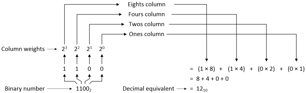
Combining digits with column weights in binary (Source: Max Maxfield)

Observe that we’ve used ‘2’ and ‘10’ subscripts to reflect the binary and decimal nature of the numbers, respectively. By convention, unless otherwise indicated by the context, a number without a subscript is assumed to be in base-10. This is similar to the way in which we assume a decimal number like 24 to be a positive value, so we don’t feel the need to include the plus sign and write +24.

Natural Numbers, Whole Numbers, and Integers

In mathematics, the term natural numbers (a.k.a. counting numbers) refers to the positive numbers we use to count from 1 to infinity. The set of natural numbers is usually denoted by the symbol N, where N = {1, 2, 3, 4, 5…∞}. Meanwhile, the term whole numbers refers to the combination of the set of natural numbers and the number zero. The set of whole numbers is usually denoted by the symbol W, where W = {0, 1, 2, 3, 4, 5…∞}.

The term integers refers to the set comprising all the negative counting numbers, zero, and all the positive counting numbers. The set of integers is usually denoted by the symbol Z, where Z = {-∞…-5, -4, -3, -2, -1, 0, 1, 2, 3, 4, 5…∞}.

So, what do computer geeks mean when they use the expression positive integers? To be honest, this is a tricky one. According to mathematicians, the positive integers embrace only those integers that are accompanied by a plus sign, which—as we previously noted—doesn’t actually need to be written by convention. Since zero isn’t positive or negative per se, this means mathematicians equate positive integers with natural numbers (i.e., excluding zero).

However, many people consider zero to be a positive integer on the basis that it doesn’t carry a minus sign (“not being negative makes it positive,” as it were). This is the view (albeit unconsciously) adopted by most members of the computing community. As a result, computer nerds typically equate positive integers with whole numbers (i.e., including zero), and this is the definition we will adopt going forward.

Bits, Bytes, and Nybbles

As we previously noted, the smallest unit of binary data is a bit (binary digit). If one bit can represent two values, 0 and 1, then a group of two bits can be used to represent 2² = 2 x 2 = four values: 00, 01, 10, and 11. Similarly, a group of three bits can be used to represent 2³ = 2 x 2 x 2 = eight values: 000, 001, 010, 011, 100, 101, 110, and 111.

A common grouping is called a nybble (or nibble), which comprises four bits. These bits can be used to represent 2⁴ = 16 different binary patterns of 0s and 1s from 0000 to 1111. If we decide to use these 16 patterns to indicate only positive integers, then we can represent values from 0 to 15 in decimal.

Another common grouping is called a byte, which comprises eight bits. Thus, “two nybbles make a byte,” which is a computer geek’s idea of an outrageously funny play on words. These bits can be used to represent 2⁸ = 256 different binary patterns of 0s and 1s from 00000000 to 11111111. If we decide to use these 256 patterns to reflect only positive integers, then we can represent values from 0 to 255 in decimal.

Leading Zeros

Decimal numbers written using pencil and paper can be arbitrarily large depending on the number of pencils at your disposal and your stamina. By comparison, the maximum value of a number in a digital computer is restricted by the number of bits that are available to represent it.

When writing binary numbers, we usually employ leading zeros—that is, 0s in the most-significant (left-hand side) bit positions—to pad binary numbers to reflect the size of the fields used to represent them in the computer. For example, the binary values 0110 and 00000110 are both equivalent to 6 in decimal, but—based on the number of leading zeros—we know that the former will be transported, manipulated, and stored as a 4-bit nybble, while the latter will be transported, manipulated, and stored as an 8-bit byte.

Switches and Relays

During the first few decades of the 20th century, engineers and inventors started to realize that electric circuits could offer the ability to perform arithmetic functions and/or execute sequences of operations to control things like industrial machinery.

Consider a simple circuit formed from a battery, a light bulb, and two single pole, single throw (SPST) switches (like traditional light switches) as depicted in the illustration below.

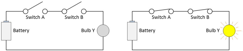
Using ON/OFF switches to implement an AND function (Source: Max Maxfield)

In this case, the switches are connected in series (one after the other) and the light will only be ON if both of the switches are CLOSED. Today, we would recognize this as being the switch-level implementation of a logical AND function, but this terminology was unknown to the folks back then.

Now consider a variation of our original circuit in which the switches are connected in parallel (side-by-side) as illustrated below.

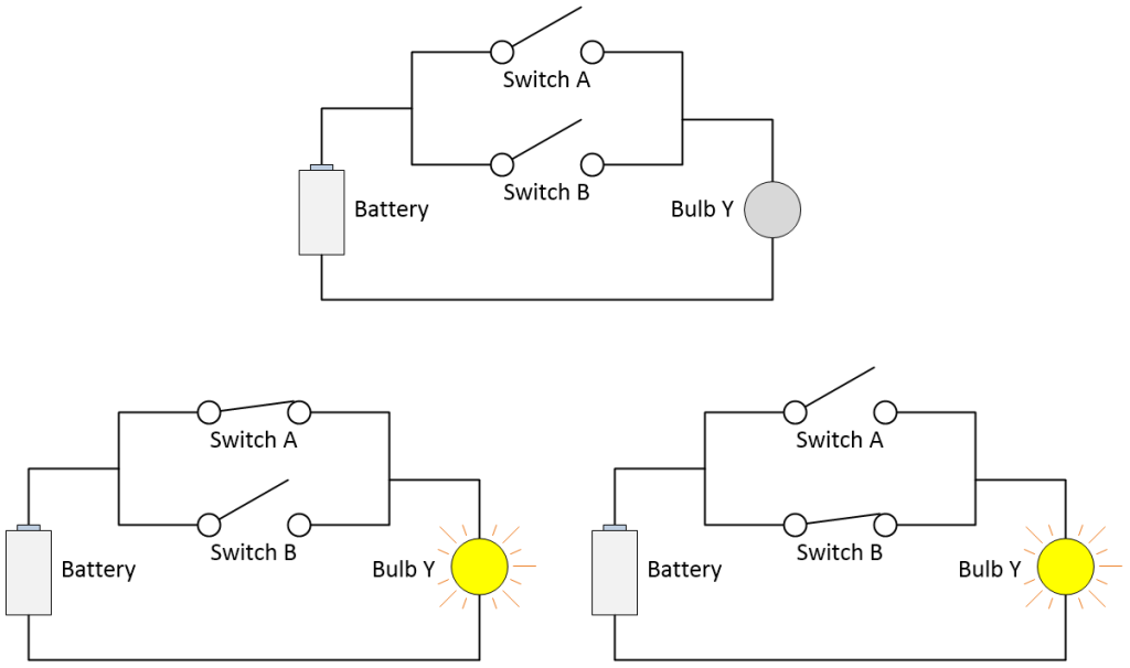
Using ON/OFF switches to implement an OR function (Source: Max Maxfield)

In this case, the light will be ON if either of the switches is CLOSED (it will also be ON if both of the switches are CLOSED). Today, we would recognize this as the switch-level implementation of a logical OR function, but—once again—the folks in the early part of the 20th century were not familiar with this terminology.

It’s possible to implement arbitrarily complex logical functions by connecting lots of switches together in different ways. These functions can have multiple inputs and multiple outputs. As opposed to the inputs being switches controlled by humans, they could be activated and deactivated by other means, such as a moving part of a machine, for example. Similarly, as an alternative to light bulbs, the outputs could be actuators like electric motors.

The thing about hand-operated switches is that it takes a relatively long time for a human to decide what needs to be done and to do it. One alternative that started to be employed circa the early 1930s was to replace hand-operated switches with their electromechanical counterparts in the form of relays, the first versions of which were introduced approximately 100 years earlier around the mid-1830s.

A traditional relay employs an electromagnet consisting of a coil of wire wrapped around an iron (ferromagnetic) core. Applying an electric potential across the ends of the coil generates an electromagnetic field that can be used to close or open associated switch contacts.

Since relays are switches, the terminology applied to regular switches also applies to relays. For example, a relay switches one or more poles, each of whose contacts can be thrown by energizing the coil. Normally open (NO) contacts connect the circuit when the relay is activated; the circuit is disconnected when the relay is inactive. Normally closed (NC) contacts disconnect the circuit when the relay is activated; the circuit is connected when the relay is inactive.

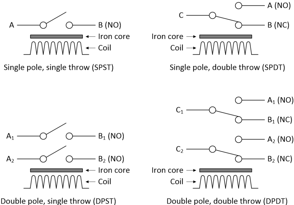
Circuit symbols for simple relays (C denotes the common terminal in SPDT and DPDT types)
(Source: Max Maxfield)

Where things start to get really interesting is that the output from one relay can activate the coil of another. This means that it’s possible to connect a bunch of relays in such a way as to implement a finite state machine (FSM) that can automatically cycle through a complex sequence of operations much faster than could be achieved if controlling switches by hand.

From one perspective, digital computers are little more than complex state machines, and some of the early digital computers circa the 1940s were implemented using relays. However, creating systems of this complexity was impractical in the early 1930s, primarily due to the fact that engineers simply didn’t have the necessary mathematical tools at their disposal.

Vacuum Tubes

In 1879, the legendary American inventor Thomas Alva Edison didn’t invent the first incandescent light bulb. It’s true that Edison did invent a light bulb, it just wasn’t the first. In 1878 (a year earlier than Edison), using a carbonized thread as a filament (the same material Edison eventually decided upon), English physicist and electrician Sir Joseph Wilson Swan successfully demonstrated a true incandescent bulb. Furthermore, in 1880, Swan gave the world’s first large-scale public exhibition of electric lamps at Newcastle, England.

In 1879, Edison publicly exhibited his incandescent electric light bulb for the first time. Edison’s light bulbs employed a conducting filament mounted in a glass bulb from which the air was evacuated leaving a vacuum. Passing electricity through the filament caused it to heat up enough to become incandescent and radiate light, while the vacuum prevented the filament from oxidizing and burning up. Edison continued to experiment with his light bulbs and, in 1883, found he could detect electrons flowing through the vacuum from the lighted filament to a metal plate mounted inside the bulb. This discovery subsequently became known as the Edison Effect.

Edison did not develop this particular finding any further, but an English physicist, John Ambrose Fleming, discovered that the Edison Effect could also be used to detect radio waves and to convert them to electricity. In 1904, Fleming developed a two-element vacuum tube known as diode.

Two years later, in 1906, the American inventor Lee de Forest introduced a third electrode called the grid into the vacuum tube. The resulting triode could be used as both an amplifier and a switch. Many of the early radio transmitters were built by de Forest using these triodes (he also presented the first live opera broadcast and the first news report on radio). In addition to revolutionizing the field of broadcasting, the ability of vacuum tubes to act as switches was to have a tremendous impact on digital computing, and many of the early digital computers circa the 1940s were implemented using these tubes.

Boolean Algebra

In order to set the scene, let’s start by noting that the term proposition refers to a statement or assertion that expresses a judgment or opinion that is either true or false. The proposition, “I just poured a bucket of burning oil in your lap,” for example, may be true or it may be false, but there’s certainly no ambiguity about it.

Sometime around the 1850s, a British mathematician called George Boole established a new mathematical field known as symbolic logic in which the logical relationships between propositions can be represented symbolically using equations.

Propositions can be combined in several ways, including conjunctions and disjunctions. A conjunction refers to propositions combined with an AND operator; for example, “You have a parrot on your head AND you have a fish in your ear.” The result of a conjunction is true only if all of the propositions comprising that conjunction are true, otherwise the result is false. By comparison, a disjunction refers to propositions combined with an OR operator; for example, “You have a parrot on your head OR you have a fish in your ear.” The result of a disjunction is true if at least one of the propositions comprising that disjunction is true, otherwise the result is false.

Boole’s work remained largely unknown outside mathematical circles until the late 1930s, at which time a graduate student at MIT called Claude Elwood Shannon submitted a master’s thesis that revolutionized electronics. In this thesis, Shannon showed that Boolean algebra offered an ideal technique for representing the logical operation of digital systems. Shannon had realized that the Boolean concepts of false and true could be mapped onto the binary digits 0 and 1, and that both could be easily implemented by means of electronic circuits.

Truth Tables

Another weapon in the digital design engineer’s arsenal is the concept of truth tables. Somewhat surprisingly, although they are intimately related to Boolean algebra, truth tables weren’t invented by Boole himself.

Dating from 1893, the first known example of truth tables was found in unpublished manuscripts by the American philosopher, logician, mathematician, and scientist Charles Sanders Peirce. However, it’s the Austrian-British philosopher Ludwig Josef Johann Wittgenstein who is generally credited with inventing and popularizing the truth table in his Tractatus Logico-Philosophicus, which was completed in 1918 and published in 1921. Also in 1921, a similar system was independently proposed by American mathematician and logician Emil Leon Post.

A truth table has one column for each input variable and one column for each output variable. Each variable can have one of two values: F (false) or T (true). Each row of the truth table contains one possible configuration of the input variables, along with the results of the operation for those values, which are reflected in the columns associated with the output variables.

Consider a function with two input variables ‘a’ and ‘b’ and one output variable ‘y’. As there are two input variables, and since each input variable can have two values, F or T, this means there are 2² = 4 possible row permutations associated with the input variables: FF, FT, TF, and TT. Furthermore, since there are four rows, this means there are 2⁴ = 16 unique permutations of outputs, whose columns we might indicate as y₀ through y₁₅.

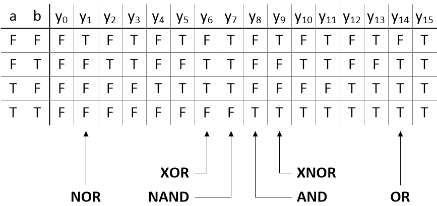
A 2-input truth table has 16 possible combinations of outputs
(Source: Max Maxfield)

As depicted above, the original truth tables employed F and T to represent false and true, respectively. This may be suitable for students of symbolic logic and acceptable to adherents of propositional calculus, but digital logic designers like your humble narrator find it makes our heads hurt if we look at these too long. Thus, henceforth, we will skip forward to the time when engineers started to use 0 and 1 to represent F and T, respectively.

Out of the sixteen permutations shown above, there are six that electronic engineers predominantly use. We call these AND, NAND, OR, NOR, XOR, and XNOR. 

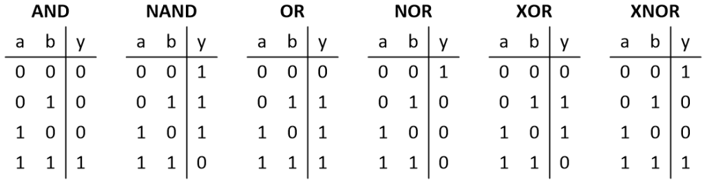
Truth tables for 2-input AND, NAND, OR, NOR, XOR, and XNOR functions (Source: Max Maxfield)

Remember that we are using 0 to represent false and 1 to represent true. In the case of an AND, the output is true only when both inputs are true, otherwise the output is false. In the case of an OR (which is more properly referred to as an “inclusive OR”), the output is true if either of the inputs are true (including the case where both inputs are true), otherwise the output is false. Contrast this with the XOR (“exclusive OR”), in which the output is true if either of the inputs are true (excluding the case where both inputs are true), otherwise the output is false.

In the case of the NAND (“not AND”), NOR (“not OR), and XNOR (“exclusive NOR”) functions, the outputs are the logical inversions of those for the AND, OR, and XOR, respectively.

As a point of interest, logic functions like AND, NAND, OR, NOR, XOR, and XNOR can be realized in a variety of implementation technologies. In addition to electrical switches, electromechanical relays, and vacuum tubes as introduced above, along with semiconductor devices like transistors as discussed below, these functions can be implemented using mechanical, hydraulic, and pneumatic means, to name but a few possibilities (see my column on the marble-based Turing Tumble, for example).

Transistors and Logic Gates

When it comes to electricity, most materials are conductors, insulators, or something in-between, but a special class of materials called semiconductors can be persuaded to exhibit both conducting and insulating properties. Silicon is one such material.

A transistor is a three-terminal semiconductor device. The first transistor, a point-contact component, was created in 1947. A more reliable version known as a bipolar junction transistor (BJT) was invented in 1950, and another implementation known as a field-effect transistor (FET) was introduced in 1960.

In the analog world, a transistor can be used as a voltage amplifier, a current amplifier, or a switch. In the digital domain, which is our area of interest here, a transistor is primarily considered to be a switch. Consider a regular toggle switch compared to a FET.

Toggle switch (left) and transistor (right) (Source: Max Maxfield)

Closing the switch and making the connection allows electricity to flow between its A and B terminals, while opening the switch and breaking the connection prevents the flow of electricity between the A and B terminals. Similarly, in the case of the transistor, an electric potential applied to its control terminal can be used to turn the transistor on, thereby allowing electricity to flow between its A and B terminals. Contrariwise, removing the potential from the control terminal will turn the transistor off, thereby preventing the flow of electricity between the A and B terminals.

One difference between a mechanical switch and a transistor switch is size. Mechanical switches are relatively large, but it’s now possible for us to fabricate transistors so small that we can create billions of them on a single silicon chip. Another difference is speed. A mechanical switch takes a relatively long time to operate, while transistor switches can be activated and deactivated millions or billions of times a second. Moreover, mechanical switches have to be operated by people (or by some similar means), while transistors can be controlled by other transistors, which allows us to create super-fast and super-sophisticated electronic systems. 

One thing we can do with transistors is connect them together to implement logic functions like the AND, NAND, OR, NOR, XOR, and XNOR functions we introduced earlier. Let’s take the AND, for example. We could regard this in electrical terms as a black box with +ve (power) and 0V (ground) connections. In this case, we might also consider the values on its input and output signals in terms of +ve and 0V as illustrated below.

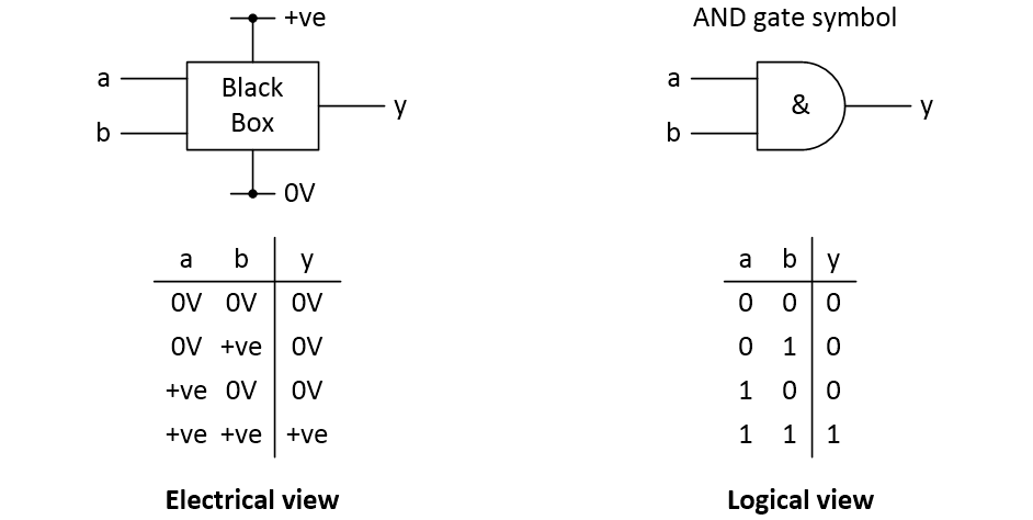
Electrical vs. logical views of an AND function (Source: Max Maxfield)

If we knew what voltage our computer was using—say 5V, for example—we could substitute this value in our electrical truth table. The problem is that different computers use different voltages and things can easily become confusing. It makes our lives so much simpler to work in an abstract world of logic gate symbols and logical 0 and 1 values.

Speaking of which, thus far we’ve primarily talked about logic functions. Simple functions such as AND, NAND, OR, NOR, XOR, and XNOR are often known as primitive gates, primitives, logic gates, or simply gates. These simple gates can be combined to implement more complex functions.

Strictly speaking, the term logic function implies an abstract mathematical relationship, while logic gate suggests an underlying physical implementation. In practice, however, these terms are often used interchangeably. The reasoning underlying the “gate” nomenclature is that a gate refers to anything that allows or prevents passage. Similarly, logic gates allow or prevent the passage of signals.

Zeros and Ones

We started this column by saying: “It’s common to hear engineers and computer boffins say that digital computers are based on 0s and 1s, but what does this actually mean?” I dare to hope we’re now in a better position to answer that question.

On the hardware side, it’s relatively easy for us to use transistors to create electronic implementations of simple logic gates like AND, NAND, OR, NOR, XOR, and XNOR that can detect the difference between two different voltages on their inputs and generate two different voltages on their outputs. Rather than talk in terms of specific voltage values, we abstract them and refer to them as 0 and 1. We can also create memory elements that can store our 0 and 1 values.

We can use our simple gates and memory elements to create larger functions, which we can employ to perform both arithmetic and logical operations. One such function is called a finite state machine (FSM), which is an abstract machine that can be in one of a finite number of states at any given time. The FSM can change from one state to another in response to its inputs. A digital computer is essentially a complex FSM.

As we’ve previously discussed, the term bit refers to a binary digit, which can be used to represent 0 or 1. We can gather groups of bits together to represent pretty much anything we want. For example, we can use groups of bits to represent numerical values in the form of integers or floating-point numbers. Alternatively, we can use groups of bits to represent alphanumeric characters and punctuation symbols. In the case of the American Standard Code for Information Interchange (ASCII), for example: 01000001 represents ‘A’, 01000010 represents ‘B’, 01000001 represents ‘C’, etc. Similarly, 00110000 represents ‘0’ (the character, not the number), 00110001 represents ‘1’, 00110010 represents ‘2’, etc.

We create programs for digital computing platforms, such as the Arduino, using an integrated development environment (IDE). In the case of the Arduino, we use the C/C++ programming languages to capture a human-readable (source code) version of our program. We then use a compiler to translate this source code into the machine code equivalent that will run on the computer. This machine code, which comprises a mix of instructions and data, is presented as the 0s and 1s that can be used by the computer.

When 0s and 1s Meet the Real World

The Arduino’s IDE comes equipped with a library of built-in functions that we can call in our programs. One such function is called digitalWrite(), which can be used to write 0 or 1 values to a specified digital input/output (I/O) pin. If we wish to write a 0 to pin 6, for example, we could do so using:

    digitalWrite(6, 0);

Alternatively, if we wish to write a 1 to pin 6, we could do so using:

    digitalWrite(6, 1);

What do 0 and 1 mean in this context? Well, in the real world, they will appear as voltage values on the Arduino’s output pin. In the case of an Arduino Uno, for example, 0 and 1 will appear on the output pin as 0V and 5V, respectively. One way to visualize how this works is illustrated below.

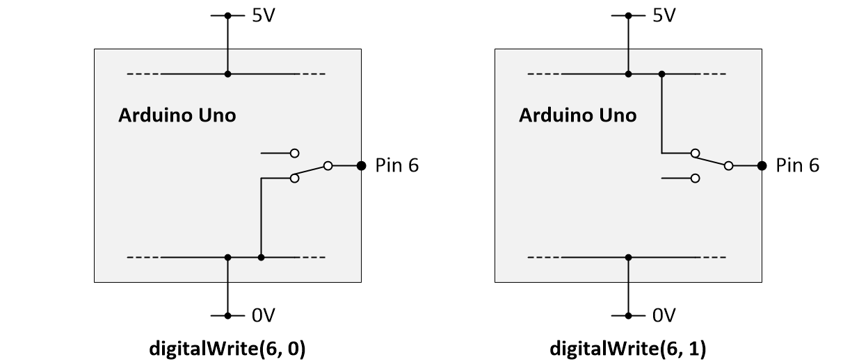
Visualizing how the Arduino’s digitalWrite() function works
(Source: Max Maxfield)

The Arduino Uno is powered by a 5V supply rail and a 0V ground rail. We can think of these rails as being replicated inside the device. Remembering that we can view a transistor as a switch, we can use a couple of transistors to implement the equivalent of a single pole, double throw (SPDT) switch. When we use a digitalWrite(6, 0) statement, this connects pin 6 to the 0V rail inside the Arduino, and this is the value that is presented to the outside world. Contrariwise, when we use a digitalWrite(6, 1) statement, this connects pin 6 to the 5V rail inside the Arduino, and it’s this value that’s presented to the outside world.

LOW and HIGH

One of the first things beginners to the Arduino are instructed to do is to use digitalWrite() commands to flash a light-emitting diode (LED) that’s connected to pin 13 on the Arduino development board. As part of this, instead of using digitalWrite(13, 0), they are told to use digitalWrite(13, LOW). Similarly, as opposed to using digitalWrite(13, 1), they are told to use digitalWrite(13, HIGH).

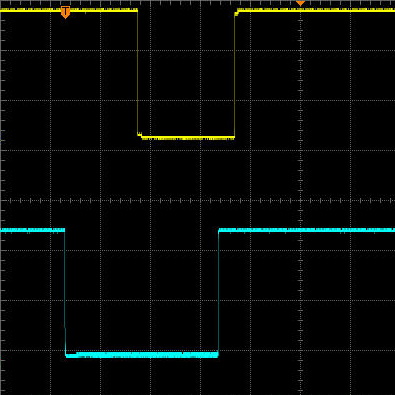
On the one hand, the terms LOW and HIGH are fairly intuitive. We can think of them as representing low and high voltages, such as 0V and 5V, for example. Consider the following screenshot from an oscilloscope:

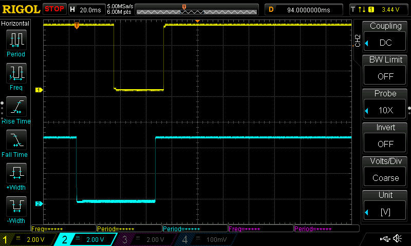
Reading from left-to-right, the yellow and blue traces both start off at 5V. After some time, the blue trace drops to 0V followed by the yellow trace. Next, the blue trace returns to 5V followed by the yellow trace. In this case, it instinctively makes sense that the more positive potential (5V, in this case) is “higher” than the more negative potential (0V, in this case).

The only problem is that the C/C++ programming languages don’t have the concept of LOW and HIGH, so where did these keywords come from?

Let’s come at this from a different direction. Suppose you were working with C/C++ in an environment that didn’t support the LOW and HIGH keywords, but you really, really wanted to use these little scamps. One solution would be to use #define preprocessor directives as follows:

    #define LOW  0
    #define HIGH 1

In fact, something akin to this is pretty much what the folks who set up the Arduino IDE did behind the scenes. I’m not exactly sure why they did this. I’m assuming it was because they thought that using LOW and HIGH would be more intuitive (and less scary) to beginners than using 0 and 1.

False and True

In computer science, the bool and boolean data types, which are named after George Boole, can have one of two possible values that are intended to represent the true and false values associated with logic and Boolean algebra.

Different programming languages support various flavors of the bool and boolean data types. Trying to wrap your brain around this topic can make your brain ache. For example, C doesn’t support a native bool data type, but you can add this type by including the “stdbool.h” header file. By comparison, C++ does support a native bool type. Neither C nor C++ support a boolean data type, but the Arduino IDE supports both types (we can think of the boolean data type as being an alias for the bool data type).

Beginners are taught that a variable of type bool or boolean can be assigned values of true and false. Although what I’m about to tell you isn’t strictly true (no pun intended), we can think of the bool data type as being an alias for the int (integer) data type. Also, although the underlying implementation is not what I’m about to show you, we can think of the false and true values as being defined in a similar way to the LOW and HIGH values, as follows:

    #define false  0
    #define true   1

This opens the door to a wide range of possibilities. For example, if we wish to write a 0 to pin 6, we could do so using:

    digitalWrite(6, false);

Alternatively, if we wish to write a 1 to pin 6, we could do so using:

    digitalWrite(6, true);

Similarly, if we declare a variable as being of type bool or boolean, in addition to assigning it values of false and true, we can also assign it values of 0 and 1 and LOW and HIGH.

In Conclusion

As I mentioned at the beginning of this column: “There are so many layers to this metaphorical onion that, much like a corporeal onion, it can make your eyes water.” Are your eyes watering yet?

If the truth be told (again, no pun intended), we’ve only scratched the surface of this topic. Hopefully, however, I’ve managed to convince you that digital computers are based on 0s and 1s, and that everything else ultimately resolves into these two values. If so, you will be distressed to learn that this is not actually 100% of the case 100% of the time, but—for the sake of our collective sanity—we will leave talk about topics like trits, trytes, trybbles and ternary computers for a future column.

Until then, as always, I welcome your insightful comments, perspicacious questions, and sagacious suggestions.