

With most of the articles I write, I try to do more than just parrot what someone else said: I really try to understand what it is I’m writing about, at least to some degree.
Not today, folks.
Not even close.
Today we go behind the looking glass into the world of quantum computing. I’m going to try to give a flavor of what I’ve learned in order to understand what’s significant about the news coming out of the University of California at Santa Barbara (UCSB), but I’m not even going to try to pretend that I really know what I’m talking about.
When interviewing the UCSB team, they tossed about concepts with deceptive ease; on the one hand, it seemed like I should have been able to follow along easily, but, on the other hand, it felt like I was in one of those bad dreams where I forgot that I had signed up for a quantum class – and I’m just realizing that the final is today and I totally need to fake it.
So we’ll work through this to a point, although I feel like, at any second, my thoughts may spontaneously decohere.
In theory
Where to start? Let’s go basic and then work up from there. As you may well know, the whole idea of quantum computing begins with the concept of superposition. Think Schroedinger’s cat, simultaneously alive and dead – until we peer into the box, at which point the superposition collapses into a specific state. In the computing case, we start with the basic unit of… logic (if you can call it that): the qubit.
An ideal qubit can have a state 1 or 0. Or… it can simultaneously be 1 and 0. Seriously. The benefit of this otherwise dubious-sounding characteristic is that computations are performed on all superimposed states simultaneously, akin to a massively parallel system. For certain (although not all) problems, this can be a big win.
But it’s not as simple as 1 or 0 or some value in between. Oh no, that wouldn’t be nearly eerie enough. The states are actually complex, represented by what’s referred to as a “Bloch Sphere.”

Image credit: Glosser.ca (Wikipedia)
A couple of things here you may notice right away: we can’t use simple letters and numbers to indicate variables and states; no, we gotta get all fancy and put hats on the variables and surround the state with characters that are hard to find in the symbols dialog.
Here we see variable z? (you can’t even find that in a font – you have to use combining diacritics! [Editorial note much later: we did a complete change to our web hosting, and the new system doesn’t appear to represent these goofy characters correctly. Only the vertical lines show; not the side brackets, and no hats. Apologies…] They don’t even use that in the Balkans, where they invert the hat). When vertical, it’s considered to be in state 0, which we can’t call state 0, since that would obviously be too easy – we have to call it |0?. I’m sure there’s a good reason for that.
Flip the state of the vector upside down, and now we’ve got state |1?. So far so good. But here’s where the good bits start: rotate the vector only 90° and you have a superimposed |1?/|0? state. But, because this is a sphere, there are obviously lots of ways to have this state, depending on where along the equator the vector ends up pointing. Thanks to this phase element, the state is, in fact, a complex entity (in the mathematical sense, not in – or in addition to – the sense of having blown bits of my brain away).
So, in a dramatically over-simplified way, computing operations consist of implementing these rotations on groups of qubits in a coherent way. Meaning they’re entangled, mangling all their states together. Measuring the result causes all the superposition to collapse and you get an answer. Which will hopefully be the right answer.
“Hopefully” because this isn’t a precise, deterministic thing going on. (I guess that, thanks to Heisenberg, there’s nothing about quantum that can be considered to be “precise”…) There are various sorts of error, even in an ideal case. The rotations might be slightly off, the system might slowly decohere, and, even if none of that happens, there’s a chance that, when you read the answer, it will be wrong. “Ha ha! Just kidding!! The cat was actually alive. Sorry about those scratches on your arm…”
We’ll come back to sources of error shortly, but the point for now is that reliability is a big problem. You might say it’s THE big problem. We’re used to increasing levels of error in standard circuits due to noise or alpha particles or what-not, and we use error correction to handle that. Why not use that for unreliable quantum systems as well? In fact, that’s the goal. But, in order to do that, the overall uncorrected reliability has to be greater than 99%: above that point, error correction can get you the rest of the way.
Getting to 99% has been hard. Which is why we’re having this little chat.
Getting real
So far, we’ve been talking theoretical niceties. The next obvious question is, how do you build one of these things in real life? There are lots of approaches that have been tried; we’ll focus on UCSB’s approach. They call their qubit implementation a “transmon.” (Which, given my mental state working through this stuff, belongs in a sentence such as a Caribbean, “I’m in a trance, mon.”)
It’s fundamentally an LC tank. The capacitor is in a distinctive cross shape. The inductors aren’t really visible: they’re tiny Josephson junctions. Which need to be operated at cryogenic temperatures. Like… 30 mK. 30 thousandths of a Kelvin above absolute zero. Frickin’ brrr.
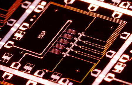
Image courtesy UCSB; credit Erik Lucero
You’ll notice there are five crosses in a row: this is a five-qubit system. Each one can be addressed and manipulated through “tones.” This is a microwave system, so the tones consist of specific frequencies. The amplitude-time product (basically, energy) is the operative parameter. Specific values can drive a qubit to a |1? or a |0? state; going half-way gets you to a superimposed |1?/|0? state.
In order to make the qubits addressable, they used a “ladder” of tones with irregular spacing between the “rungs” so that no qubit would accidentally respond to another qubit’s tone.
The overall system includes resonators for reading (those squiggly lines you see), x and y control lines to which voltage pulses are applied for phase rotations, and a z line for current pulses. The z line – oddly, to this traditional circuit guy – has no return path… it’s used to create a magnetic field that controls a tunable inductor formed out of a ring with two superconducting Josephson junctions… and I’m just accepting that and running with it. Kirchoff, you lied…
Let’s come back to the possible sources of error that can keep the overall reliability below 99%. We saw that some are intrinsic, occurring even in an ideal system. Creating a real-world physical system only makes that worse by introducing more sources of error.
Here’s the hit parade of quantum computing nemeses:
- Dephasing: this is an odd one; it amounts to phase jitter as the system experiences noise. The qubits can come out of phase with respect to each other, some moving one way, some another in a kind of “spread.” (There’s a clever trick for reversing this: apply a 180° rotation and the “spreading” action brings the vectors back into coherence. My analogy is like watching a road race: everyone is together at the start, but the group spreads out as faster runners advance and slower ones lag. To get them all back together again, simply tell them all to turn around. The faster guys, now behind, will catch up to the slower ones, and, eventually, the group reforms.)
- Parasitic coupling to defects in the materials.
- Noise on the control lines.
- Energy loss:
- Microwave dissipation, which is vanishingly small, but not zero.
- Capacitor dielectric defects.
- Slight errors when establishing the superimposed state. Ideally, you want a 50/50 mix of |1? and |0?, but you may get something like 49.9/50.1.
- Slight errors when applying phase rotations.
- Cross-talk between qubits.
- And, even if all of these sources are eliminated, there’s always the random chance of getting the wrong answer when reading the result.
The use of redundant qubits and error-correcting “surface codes” are tools aimed at making these systems reliable enough for commercial use. The system built by the team didn’t use redundant bits (that’s for future work), but they did use surface codes, and their result was 99.92% reliability for a single qubit and 99.4% for two qubits.
Which, presumably, was cause for great celebration. Perhaps loud enough to wake the cat. If, that is, the cat was truly alive and merely sleeping. Which, of course, we’ll never really know for sure…
(Yes, we occasionally – rarely, actually – do kittehs on EE Journal. No need to LOL. At least it’s not cute. You’re welcome.)


Does quantum computing scramble your brain as much as it does mine?